Tutorial#
Tutorial Preliminaries: Data Preparation and Helpers
To follow the example here, install the necessary dependencies:
uv pip install volara[docs]
import random
import pprint

import matplotlib.pyplot as plt
import numpy as np
from funlib.geometry import Coordinate
from funlib.persistence import prepare_ds
from scipy.ndimage import label
from skimage import data
from skimage.filters import gaussian

from volara.tmp import seg_to_affgraph

# Download the data
cell_data = (data.cells3d().transpose((1, 0, 2, 3)) / 256).astype(np.uint8)

# Handle metadata
offset = Coordinate(0, 0, 0)
voxel_size = Coordinate(290, 260, 260)
axis_names = ["c^", "z", "y", "x"]
units = ["nm", "nm", "nm"]

# Create the zarr array with appropriate metadata
cell_array = prepare_ds(
    "cells3d.zarr/raw",
    cell_data.shape,
    offset=offset,
    voxel_size=voxel_size,
    axis_names=axis_names,
    units=units,
    mode="w",
    dtype=np.uint8,
)

# Save the cell data to the zarr array
cell_array[:] = cell_data

# Generate and save some pseudo ground truth data
mask_array = prepare_ds(
    "cells3d.zarr/mask",
    cell_data.shape[1:],
    offset=offset,
    voxel_size=voxel_size,
    axis_names=axis_names[1:],
    units=units,
    mode="w",
    dtype=np.uint8,
)
cell_mask = np.clip(gaussian(cell_data[1] / 255.0, sigma=1), 0, 255) * 255 > 30
not_membrane_mask = np.clip(gaussian(cell_data[0] / 255.0, sigma=1), 0, 255) * 255 < 10
mask_array[:] = cell_mask * not_membrane_mask

# Generate labels via connected components
labels_array = prepare_ds(
    "cells3d.zarr/labels",
    cell_data.shape[1:],
    offset=offset,
    voxel_size=voxel_size,
    axis_names=axis_names[1:],
    units=units,
    mode="w",
    dtype=np.uint8,
)
labels_array[:] = label(mask_array[:])[0]

# Generate affinity graph
affs_array = prepare_ds(
    "cells3d.zarr/affs",
    (3,) + cell_data.shape[1:],
    offset=offset,
    voxel_size=voxel_size,
    axis_names=["offset^"] + axis_names[1:],
    units=units,
    mode="w",
    dtype=np.uint8,
)
affs_array[:] = (
    seg_to_affgraph(labels_array[:], nhood=[[1, 0, 0], [0, 1, 0], [0, 0, 1]]) * 255
)


# Helper function to show an image, channels first
def imshow(data):
    if data.shape[0] == 2 and len(data.shape) == 3:
        data = data[[0, 1, 0]] * np.array([1, 1, 0]).reshape(3, 1, 1)
    if data.dtype == np.uint32 or data.dtype == np.uint64:
        labels = [x for x in np.unique(data) if x != 0]
        relabelling = random.sample(range(1, len(labels) + 1), len(labels))
        for l, new_l in zip(labels, relabelling):
            data[data == l] = new_l
        cmap = "jet"
    else:
        cmap = None

    fig = plt.figure(figsize=(10, 4))
    if len(data.shape) <= 3:
        if len(data.shape) == 2:
            plt.imshow(data, cmap=cmap, interpolation="none")
        else:
            plt.imshow(data.transpose(1, 2, 0), cmap=cmap, interpolation="none")
    plt.show()
Introduction#
In this tutorial, we will demonstrate the usefulness of this library for processing large image data in the context of instance segmentation. We will use some very simple toy data to dive into more detail of how to use volara and what you get when running some basic operations.
Viewing Data#
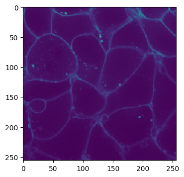
A 2D slice of the data we are working with is shown below.
Channel 0:
imshow(cell_array[0, 30])
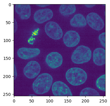
Channel 1:
imshow(cell_array[1, 30])
Both Channels:
imshow(cell_array[:, 30])
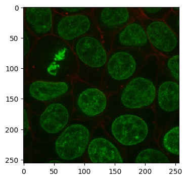
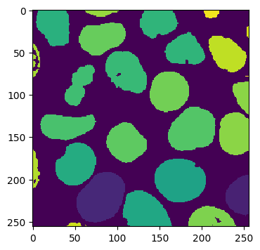
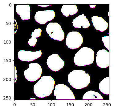
As you can see, the volume we are working with is a two-channel fluorescence image of nuclei and cell membranes. We have also generated some pseudo ground truth via some simple blurring and thresholding:
Pseudo Ground Truth:
imshow(labels_array[30])
All of this data is stored in a zarr container cells3d.zarr. We created each
array with some helpful metadata such as the offset, voxel size, axis names, and
units. This is not necessary for processing but is good bookkeeping practice.
The raw data is a 2-channel image, with a resolution of 0.29x0.26x0.26 microns.
We have chosen to name the axes as c^, z, y, and x. The ground truth
has the same metadata. The ground truth should normally be manually curated to
ensure quality, but this will be fine for our purposes.
Finally, we have also gone ahead and generated affinities from the ground truth
labels. This is commonly done with a machine learning model (UNet) when trying to
generate an instance segmentation. We will be working with perfect affinities for
this tutorial but most applications will be a bit noisier.
Affinities:
imshow(affs_array[:, 30])
Generating Supervoxels#
Now we get to using volara. Our goal will be to take the “model predictions”, i.e., the affinities, and generate something like the ground truth segmentation. volara allows us to do this in a blockwise way which becomes necessary as soon as you leave the realm of toy data.
First, we need to generate supervoxels from the affinities. This can be done by running a watershed within each chunk we process.
from volara.blockwise import ExtractFrags
from volara.datasets import Affs, Labels
from volara.dbs import SQLite

# Configure your db
db = SQLite(
    path="cells3d.zarr/db.sqlite",
    edge_attrs={
        "zyx_aff": "float",
    },
)

# Configure your arrays
affinities = Affs(
    store="cells3d.zarr/affs",
    neighborhood=[Coordinate(1, 0, 0), Coordinate(0, 1, 0), Coordinate(0, 0, 1)],
)
fragments = Labels(store="cells3d.zarr/fragments")

# Extract Fragments
extract_frags = ExtractFrags(
    db=db,
    affs_data=affinities,
    frags_data=fragments,
    block_size=(20, 100, 100),
    context=(2, 2, 2),
    bias=[-0.5, -0.5, -0.5],
)
extract_frags.run_blockwise(multiprocessing=False)
Execution Summary
-----------------

  Task fragments-extract-frags:

    num blocks : 27
    completed ✔: 27 (skipped 0)
    failed    ✗: 0
    orphaned  ∅: 0

    all blocks processed successfully
defaultdict(daisy.task_state.TaskState,
            {'fragments-extract-frags': Started: True
             Total Blocks: 27
             Ready: 0
             Processing: 0
             Pending: 0
             Completed: 27
             Skipped: 0
             Failed: 0
             Orphaned: 0})
Bias and Blockwise Operation#
Now we have supervoxels, but before we look at them, let’s talk about some of the code that went into generating the fragments. We have an argument called bias. This defines how much we want to emphasize splitting or merging. Affinities are normally generated such that 0 indicates a boundary between objects and 1 means the voxels belong to the same object. When we extract fragments, we use negative scores for splitting and positive for merging. This means a bias of -2 would split everything since even our most confident affinities would split. A bias of 1 would mean that even our most uncertain affinities would result in a merge. Finally, a bias of -0.5 shifts our affinities to the range (-0.5, 0.5), resulting in splits across boundaries and merges within objects. We provide a bias for every offset in our neighborhood, which allows us to treat offsets very differently. This can be particularly useful when you train long-range affinities since we generally see much nicer segmentations when we use long-range affinity scores for splitting and neighboring voxel affinities for merging objects.
The only other variables we had to specify other than the simple paths to the data we are working with are the block_size and context. Both are provided in voxels. A larger context will result in fragments that have more consistent edges at block boundaries, but normally does not need to be significantly larger than the max offset in your neighborhood. The block size should be set based on the compute constraints of your system.
Viewing Fragments#
Now let’s take a look at the fragments we generated:
imshow(fragments.array("r")[30])
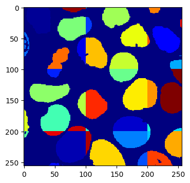
As you can see, we get a fragments array of full segmentations, which is expected given that we are working blockwise. Note that you can clearly see the block boundaries.
Fragment Graph#
One thing we still haven’t talked about is the db argument to ExtractFrags. Using a database allows us to store the fragments we generate in a way that is easy to operate on without having to load the image data at all, and reduces an operation that would be done on in this case (60x256x256) voxels to an operation done one just a few hundred nodes and edges.
fragment_graph = db.open("r").read_graph(cell_array.roi)
print(f"Number of fragments generated: {len(fragment_graph.nodes)}")
print("Some sample fragments: ")
pprint.pp(list(fragment_graph.nodes(data=True))[100:105])
Number of fragments generated: 218
Some sample fragments:
[(1800004, {'position': (11600, 4160, 22360), 'size': 15, 'filtered': None}),
 (3000004, {'position': (11600, 4420, 26000), 'size': 1, 'filtered': None}),
 (1800007, {'position': (11600, 6240, 10920), 'size': 6, 'filtered': None}),
 (3000005, {'position': (11600, 7800, 26000), 'size': 26, 'filtered': None}),
 (3000006, {'position': (11600, 10660, 42120), 'size': 2, 'filtered': None})]
As you can see, we store the fragments’ center position along with their size. You can store other attributes as well, but these attributes are always included.
Merging Fragments#
We do not yet know which fragments can be merged together to generate our final segmentation. This is obvious when we look at the edges of our fragments graph:
print(f"Number of edges in our fragment graph: {len(fragment_graph.edges)}")
Number of edges in our fragment graph: 0
Computing Edges#
Let’s compute some edges:
from volara.blockwise import AffAgglom

# Affinity Agglomeration across blocks
aff_agglom = AffAgglom(
    db=db,
    affs_data=affinities,
    frags_data=fragments,
    block_size=(20, 100, 100),
    context=(2, 2, 2),
    scores={"zyx_aff": affinities.neighborhood},
)
aff_agglom.run_blockwise(multiprocessing=False)
Execution Summary
-----------------

  Task db-aff-agglom:

    num blocks : 27
    completed ✔: 27 (skipped 0)
    failed    ✗: 0
    orphaned  ∅: 0

    all blocks processed successfully
defaultdict(daisy.task_state.TaskState,
            {'db-aff-agglom': Started: True
             Total Blocks: 27
             Ready: 0
             Processing: 0
             Pending: 0
             Completed: 27
             Skipped: 0
             Failed: 0
             Orphaned: 0})
This should have generated the edges between all pairs of fragments that are close enough to have affinities between them. Let’s take a look:
fragment_graph = db.open("r").read_graph(cell_array.roi)
print(f"Number of fragments: {len(fragment_graph.nodes)}")
print(f"Number of edges: {len(fragment_graph.edges)}")
print("Some sample edges: ")
pprint.pp(list(fragment_graph.edges(data=True))[100:105])
Number of fragments: 218
Number of edges: 137
Some sample edges:
[(2800006, 5600003, {'distance': None, 'zyx_aff': 1.0}),
 (2800008, 5600004, {'distance': None, 'zyx_aff': 1.0}),
 (600007, 1800001, {'distance': None, 'zyx_aff': 1.0}),
 (1200007, 3000003, {'distance': None, 'zyx_aff': 1.0}),
 (1200008, 3000009, {'distance': None, 'zyx_aff': 1.0})]
Global Matching and Segmentation#
Now that we have edges, we can process the graph to generate our final segmentation. This is pretty straightforward to do with mutex watershed again. We have affinity scores, we just need to make them negative for splitting edges and positive for merging edges. Thus we provide the same bias as we did during fragment agglomeration, except now passed in as a dictionary for the edge attributes we want to use:
Quick Note on Global Matching#
The global matching step is special in that we treat it like a blockwise task, but it only processes a single block containing the entire dataset. It only needs to operate on the graph of supervoxels so this is a cheap operation that can scale up to petabyte-scale datasets fairly easily. You may run into problems if you generate many millions of fragments, but using a reasonable block size and filtering out small fragments can help handle massive datasets.
from volara.blockwise import GraphMWS
from volara.lut import LUT

# Global MWS
global_mws = GraphMWS(
    db=db,
    roi=fragments.array("r").roi,
    lut=LUT(path = "cells3d.zarr/lut"),
    weights={"zyx_aff": (1.0, -0.5)},
)
global_mws.run_blockwise(multiprocessing=False)
Execution Summary
-----------------

  Task lut-graph-mws:

    num blocks : 1
    completed ✔: 1 (skipped 0)
    failed    ✗: 0
    orphaned  ∅: 0

    all blocks processed successfully
defaultdict(daisy.task_state.TaskState,
            {'lut-graph-mws': Started: True
             Total Blocks: 1
             Ready: 0
             Processing: 0
             Pending: 0
             Completed: 1
             Skipped: 0
             Failed: 0
             Orphaned: 0})
The only artifact generated by this step is a lookup table that maps fragment IDs to segment IDs. If you want to be efficient, you could load the lookup table into your favorite visualization tool and use it to color your fragments for visualization. This would be useful for exploring parameters such as different biases to see how they affect your segmentation.
Relabeling Fragments#
Once you’re happy with your segmentation, it is useful to relabel your fragments and generate a new segmentation array. Let’s do that now:
from volara.blockwise import Relabel

segments = Labels(store="cells3d.zarr/segments")

# Relabel fragments to segments using lut
relabel = Relabel(
    frags_data=fragments,
    seg_data=segments,
    lut=LUT(path="cells3d.zarr/lut"),
    block_size=(20, 100, 100),
)
relabel.run_blockwise(multiprocessing=False)
Execution Summary
-----------------

  Task segments-relabel:

    num blocks : 27
    completed ✔: 27 (skipped 0)
    failed    ✗: 0
    orphaned  ∅: 0

    all blocks processed successfully
defaultdict(daisy.task_state.TaskState,
            {'segments-relabel': Started: True
             Total Blocks: 27
             Ready: 0
             Processing: 0
             Pending: 0
             Completed: 27
             Skipped: 0
             Failed: 0
             Orphaned: 0})
Viewing Final Segmentation#
Once this completes, we can take a look at our final segmentation:
imshow(segments.array("r")[30])
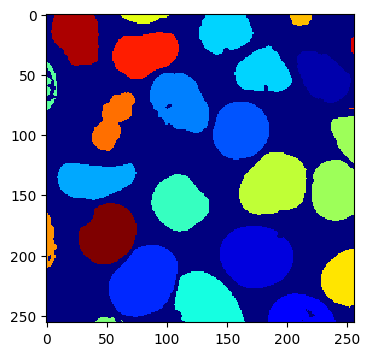
We can also check how closely this matches our original labels:
s_to_l = {}
false_merges = 0
l_to_s = {}
false_splits = 0
for s, l in zip(segments.array("r")[30].flat, labels_array[30].flat):
    if s not in s_to_l:
        s_to_l[s] = l
    elif s_to_l[s] != l:
        false_merges += 1
        print(f"Falsely merged labels: ({l}, {s_to_l[s]}) with segment {s}")
    if l not in l_to_s:
        l_to_s[l] = s
    elif l_to_s[l] != s:
        false_splits += 1
        print(f"Falsely split label: {l} into segments ({s}, {l_to_s[l]})")

print("False merges: ", false_merges)
print("False splits: ", false_splits)
print("Accuracy: ", (len(s_to_l) - (false_merges + false_splits)) / len(s_to_l))
False merges:  0
False splits:  0
Accuracy:  1.0
Our perfect accuracy is not surprising here. We used perfect affinities that were generated from the labels we were trying to reproduce.
Cleaning Up#
To clean up, let’s just remove all the data we wrote to file:
import shutil
shutil.rmtree("cells3d.zarr")
shutil.rmtree("volara_logs")